This walk through picks up where the last post left off. If you want to use these scripts with your own data, you need to have 2 data sets, each with latitude and longitude coordinates.
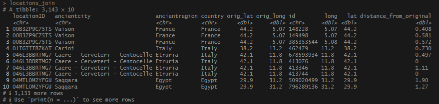
Now that I had some good location data, I wanted to use my coordinates to join the Pleiades data and see what …stuff is in the immediate area of my locations. To do this, I used a package called fuzzyjoin, which has a function called geo_inner_join (and geo_right_join, geo_left_join, etc.)* which allows you to join 2 sets of coordinates based on distance – either kilometers or miles. I decided that 2km (1.24 m) would be a good place to start. The joining took several seconds and produced a long data set with each identified each Pleiades ID on its own line.
# Read in object.
locations_master  <- readRDS(paste0(objects_directory,"locations_reversed_joined.rds"))


#attestations based on lat/long - this will take several seconds.
locations_join <- locations_master %>%
  filter(!is.na(lat)) %>%
  rename("orig_lat" = lat,
         "orig_long" = longi) %>%
  geo_inner_join(
    pleiades_from_json$pleiades_locations %>%
      filter(!is.na(long)),
    by = c("orig_long" = "long",
           "orig_lat" = "lat"),
    unit = c("km"),
    max_dist = 2,
    distance_col = "distance_from_original"
    )
Steps
- I grab the object I created a few steps ago when I performed a
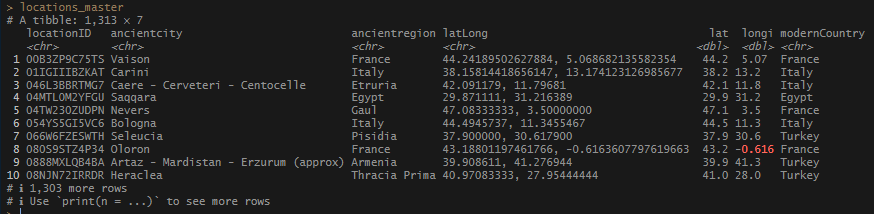
reverse_geocode()to get the modern Country names for my location. I trim it down to the columns relevant for the join and store it in an object called locations_master. - Filter out the NA values in
lat(which should remove any incomplete coordinates). - Rename my existing
lat/longcolumns so that I can easily identify which frame they belong to after I perform my join. - Perform the
geo_inner_join.- This will look at the list
pleiades_from_json$pleiades_locationsand filter out any incomplete coordinates. - Join the 2 sets: my
orig_longto Pleiades’ long, and myorig_latto Pleiades’ lat. unit = c("km")– use kilometers (km) for the units.max_dist = 2– include all matches within 2km of my coordinates.- Put the distance value in a column called “
distance_from_original“.
- This will look at the list
- Save it all in an object called
locations_join. - * – the
inner_joinindicates that the script it will keep only the records that match the requirements of the join.
Results
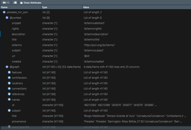
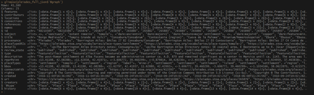
I forgot that I didn’t have names paired with those coordinates I pulled from the JSON file. Good thing I have that object at the ready. I decided to utilize the title value to give me the basic name of the record associated with the Pleiades ID’s. The pleiades_full_json$@graph$names list has every single variation on a name in Pleiades, and is a little beyond what I needed (for the moment!) I made a set of ID’s-to-titles and saved it to my pleiades_from_json_cleaned_tidied object to keep it handy. Then I joined it to locations_join.
# As before:
plei_ids <- pleiades_full_json$`@graph`$id

# Grab titles.
plei_titles <- pleiades_full_json$`@graph`$title

# Pull id's and titles together.
pleiades_titles <- tibble(
  id = plei_ids,
  plei_title = plei_titles
)

# Save these to the big list real quick.
pleiades_from_json_cleaned_tidied[["pleiades_titles"]] <- pleiades_titles

# Save the list.
saveRDS(pleiades_from_json_cleaned_tidied, paste0(objects_directory, "pleiades_from_json_cleaned_tidied.rds"))

# Join the titles to the joined set so we can see the names of the matched records.
locations_full_join_w_titles <- locations_join %>%
  left_join(
    pleiades_titles,
    by = join_by(id == id))
Steps
- Get the ID’s from
pleiades_full_json$`@graph`$id, store inplei_ids. - Extract titles list and store in
plei_titles. - Pull both sets together into one tibble called
pleiades_titles. - Save this new set to the existing
pleiades_from_json_cleaned_tidiedlist. - Join the
pleiades_titlestolocations_joinusing theidcolumn in both data sets.
Cool. Next I wanted to see which locations had the most attestations based on these coordinates.
locations_full_join_w_titles %>%
  group_by(
    ancientcity,
    country,
    orig_lat,
    orig_long
  ) %>%
  summarize(n_plei_records = n_distinct(id)) %>%
  arrange(desc(n_plei_records))
Steps
- Group the data by
ancientcity, country, orig_lat, orig_long. - Aggregate the data with
summarize()and count each distinctidin each group. Sort it so you can see the highest number of ID’s at the top. witharrange(desc()).
Results
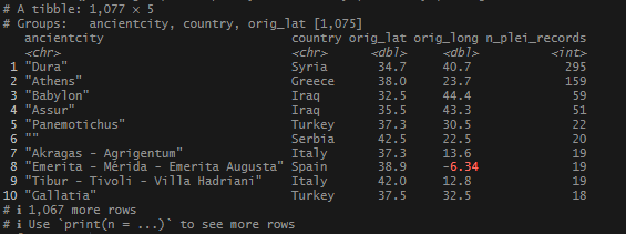
There were some famous, well attested sites that came up, but where was Rome? Or Constantinople? I decided to widen my geo_inner_join to 5km (3.11 miles), then aggregate.
locations_5km <- locations_master %>%
  filter(!is.na(lat)) %>%
  rename("orig_lat" = lat,
         "orig_long" = longi) %>%
  geo_inner_join(
    pleiades_from_json$pleiades_locations %>%
      filter(!is.na(long)),
    by = c("orig_long" = "long",
           "orig_lat" = "lat"),
    unit = c("km"),
    max_dist = 5,
    distance_col = "distance_from_original"
  )

locations_5km %>%
group_by(
  ancientcity,
  country,
  orig_lat,
  orig_long
) %>%
  summarize(n_plei_records = n_distinct(id)) %>%
  arrange(desc(n_plei_records))
These are the same steps we did before, with 5km instead of 2km.
Results
I saw more of the expected big names.
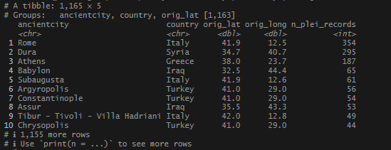
How about 10km? (Note: this code is all run together and goes right to the summary.)
locations_master %>%
  filter(!is.na(lat)) %>%
  rename("orig_lat" = lat,
         "orig_long" = longi) %>%
  geo_inner_join(
    pleiades_from_json$pleiades_locations %>%
      filter(!is.na(long)),
    by = c("orig_long" = "long",
           "orig_lat" = "lat"),
    unit = c("km"),
    max_dist = 10,
    distance_col = "distance_from_original"
  ) %>%
  group_by(
    ancientcity,
    country,
    orig_lat,
    orig_long
  ) %>%
  summarize(n_plei_records = n_distinct(id)) %>%
  arrange(desc(n_plei_records))
Results
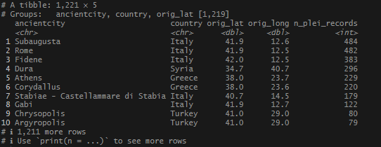
More obscure cities with tons of records. It also took a little longer to perform the join. The wider the search, the more location overlap I was likely to have. I decided that 5km might be the highest tolerance to apply in my search. And, at some point, it might be interesting to check out which ID’s my records shared in common.
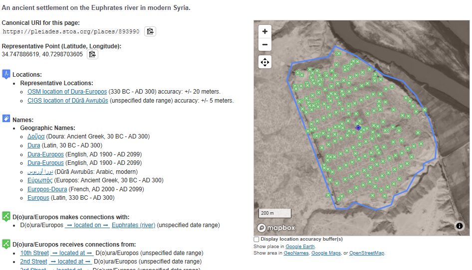
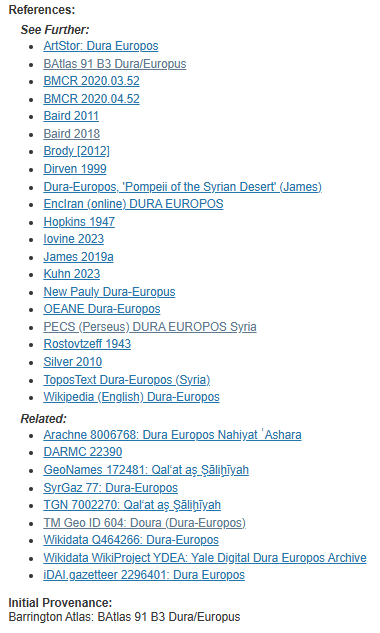
Just for fun, I checked out Dura, the 2nd most attested location. Sure enough, there is a ton of archaeological evidence and study in the region, which has produced an extensive amount of research. Pleiades links much of it in their record. What a great starting point!
Then, I wanted to check on the locations that did not produce any matches.
# Who did not have matches?
no_matches <- locations_master %>%
  left_join(locations_5km %>%
    group_by(
      locationID) %>%
      summarize(n_plei_records = n_distinct(id),
                .groups = "drop"),
    by = join_by(locationID == locationID)) %>%
  filter(is.na(n_plei_records))
Steps
- Take my original
locations_masterandleft_join()to the 5km data set. Since we just want a quick check of number of records, inside thatleft_join(), group the records tolocationIDand then get the total number of distinct Pleiades ID’s perlocationID. - Join by the
locationIDin each data set. filter(is.na(n_plei_records))to focus on the records that did not have any ID’s found for it’s coordinates.
Results
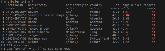
This place at the top of my NA locations, Nevers, is absolutely a real place, and when I checked, had a record in Pleiades. The problem was my coordinates were a little outside the area that Pleiades defined as the representative boundary. Really annoying. To resolve this, I decided that next I would attempt to source the data via the names. I’ll post that up when I am done working through it. The names list huge!
Finally, save the locations_5km and the locations_master objects for the next round of matches.
saveRDS(locations_5km, paste0(objects_directory,"locations_5km.rds"))
saveRDS(locations_master, paste0(objects_directory,"locations_master.rds"))
saveRDS(no_matches, paste0(objects_directory,"no_matches.rds"))
Follow along code is up on Github.
References and Resources
Robinson D (2025). fuzzyjoin: Join Tables Together on Inexact Matching. R package version 0.1.6, https://github.com/dgrtwo/fuzzyjoin.