Category: data cleaning and tidying

Once I had my long list of names, joining my no_matches set  was very easy. I used an inner_join() and pulled in any record from tris_data_long_clean that matches my locations, both in name and in country. I was able to snag several more records.

tris_matches_2_no_matches <- no_matches %>% 
  mutate(ancientcity = str_to_lower(ancientcity),
         country = str_to_lower(country)) %>%
  inner_join(
    tris_data_long_clean,
    by = join_by(ancientcity == name,
                 country == country)) 

Steps

• Apply str_to_lower() on both ancientcity and country. This helps standardize the name in case any random capitalizations exist, and assists in the inner_join().
• inner_join() to match (exactly) on the name, and also the country, to ensure we have the right place. If there is no 1:1 match on name/country, then the record will be dropped. These locations will be re-joined later.

Results

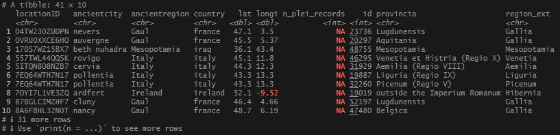
After this, I had 2 sets I wanted to bring together: locations_5km – the set joined by coordinates with Pleiades IDs; and then the new set generated from no_matches with TM IDs. I wanted to pull all of them together into one, tidy data frame. I remembered that Pleiades uses Trismegistos as one of their standard sources, and to keep things consistent, I decided to pull over the available TM ID’s from the Pleiades data. I also pulled over the Roman provincia, if it was available.

The following code, as in the post before, is broken up, but is actually one long script, meant to be run all at once.

# Start Script

# Block 1
# Bind the 2 data sets together by rows.
locations_plei_and_tris <- locations_5km %>% 
  rename("plei_id" = id) %>% 
  select(-long,
         -lat) %>% 
  bind_rows(
    tris_matches_2_no_matches %>% 
      rename("orig_lat" = lat,
             "orig_long" = longi,
             "tris_id" = id)) %>% 

Block 1

• With locations_5km, I rename the ID column to plei_id to specify that it is the Pleiades ID.
• Remove the long and lat column with select() – I only want to use my original coordinate values. I will keep the distance_from_original value for reference.
• Join the 2 sets: locations_5km and tris_matches_2_no_matches, by row with bind_rows(). This will “stack” the rows, combining like columns together, and pulling over whatever columns that are not in common between the 2 sets, and filling them with NA values. Within the bind, I clean up some column names within tris_matches_2_no_matches/

Next was a series of left_joins() to pull in the TM ID’s for the existing Pleiades ID’s I had and the provincia information for those ID’s.

  # Block 2
  left_join(
    pleiades_from_json_cleaned_tidied$pleiades_references %>% 
      filter(grepl("trismegistos", accessURI, ignore.case = T)) %>% 
      mutate(tris_id_extract = str_extract(accessURI, "[0-9]+")) %>% 
      select(id, tris_id_extract),
    by = join_by(plei_id == id)) %>% 

Block 2

• With a left_join(), I access the pleiades_references inside the JSON list, a set I made previously. The next steps are done inside the join.
  • filter() using a grepl() function. This will let you look at values in the accessURI column that contain the string “trismegistos”. I also apply ignore.case = (just to be safe). This should pull all of the Trismegistos URLs.
  • Create a new column with mutate() that will use str_extract() to pull only the ID from the URL. The "[0-9]+" is a regex expression that tells the function to only extract any number 0-9, and any additional number after it. This gives me a nice neat column with only the TM ID in tris_id_extract.
  • Select only the tris_id_extract and the (Pleiades) id.
• Finally, join the 2 sets by the ID columns.

  # Block 3
  left_join(
    tris_data_long_clean %>% 
      select(id, 
             provincia, 
             country) %>% 
      mutate(id = as.character(id)) %>% 
      distinct(),
    by = join_by(tris_id_extract == id)
  ) %>% 

Block 3

• Apply another left_join() with tris_data_long_clean (a set made in a previous step) to get the Roman provincia names. The next steps are also done inside the join.
  • Select only the id, provincia, and country columns.
  • With mutate(), convert the id to character format to facilitate the join.
  • Generate only distinct records.
• Finally, join the 2 sets by the ID columns.

  # Block 4
  mutate(trismegistos_id = coalesce(as.character(tris_id), tris_id_extract),
         trismegistos_provincia = coalesce(provincia.x, provincia.y)) %>% 
  rename("country" = country.x) %>% 
  select(-provincia.x,
         -region_ext,
         -tris_id_extract,
         -provincia.y,
         -country.y,
         -tris_id) 

# End script.

Block 4

• After the data was joined together, I have TM ID’s, in 2 columns, from the no_matches and from where I extracted the ID’s from the reference URL’s. I use coalesce() to pull them together into one column: trismegistos_id.
• Perform the same step on the provincia columns to create trismegistos_provincia.
• rename() country.x to country.
• Remove the redundant columns carried over.

Results

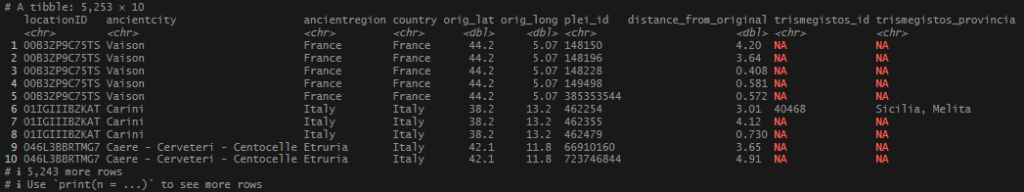
Getting close! I had all my distance-based location matches, and the extra name-based matches. I also had the TM ID’s for the Pleiades records that were pulled over on the geo_inner_join() from before. Just one more thing, pull in whatever of my original records where no location match was ever found.

locations_cited <- locations_master %>% 
  rename("orig_region" = ancientregion,
         "orig_country" = country) %>% 
  left_join(
    locations_plei_and_tris %>% 
    select(-ancientcity,
           -ancientregion,
           -country,
           -orig_lat,
           -orig_long),
    by = join_by(locationID == locationID))  

Steps

• In the original locations_master, apply better names to reflect which source the region and country came from – assign with rename().
• left_join() to the locations_plei_and_tris object that was just created. Inside the join, remove what would be redundant data. Any locationIDs that do not have a match will have NA values in both the plei_id and trismegistos_id fields.
• Join the 2 sets by locationID. Store in the object locations_cited.

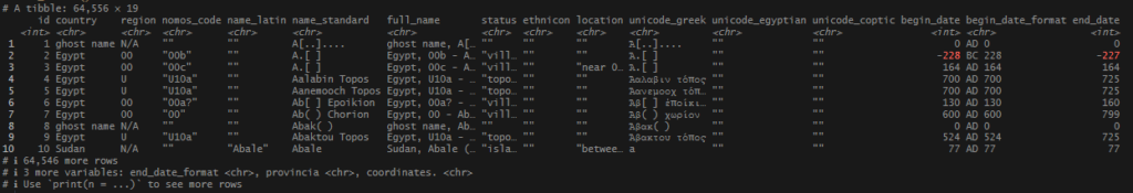
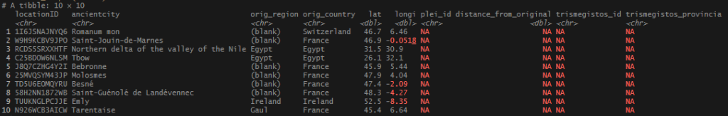
Quick look at some of the records that didn’t come over. These will require some more research or fuzzy matching to sweep them up. Fortunately, there were only 109 orphaned records out of my original set of ~1,300.

I also noticed that some of my locations independently pulled in a Pleiades ID and a TM ID, creating a duplicate row in some cases. I will have to figure out how suppress that in future iterations.

Despite that, I decided that this is really, really good locations data set, and that it would be OK to pause here and move onto something else. I was interested in taking one of my data sets, linking it to my locations data, and plotting it on a world map. Fortunately, I had a lot of other records tied to these locationID’s where I could do that.

Follow along script for parts 1 and 2 (in one file) are up on Github.

As before, this walk through picks up where the last left off. These scripts are meant to assist in separating combined fields, where unique data has been separated by 1 or more delimiters (separators). It also demonstrates pivoting data into a long format, so that it can be used in joining different data sets, based on like values, into one. I have also downloaded the .csv format of Trismegistos’ Geographical data dump to help locate names for the locations that did have matches in Pleiades. This is not a large download and requires no unzipping. They also offer the data in JSON format if you want to practice more with that.

I have the following objects loaded. These were generated in previous steps and saved as .rds files

pleiades_from_json_cleaned_tidied #Cleaned data from Pleiades JSON data
locations_5km  #Locations within 5km of the original coordinates.
locations_master #My original locations list.
no_matches #Locations that did not find a match during the fuzzyjoin.

What I wanted to do next was try to find locations that were not matched on the geo_inner_join(), and see if I could get attestations through Trismegistos (“TM” from now on) based on the name. I came to find out that was easier said than done.

The TM data was not tidy. There were multiple names, stored in many fields, across several columns. There was a composite variable (data created from combining 2 other fields): full_name that had additional info in it, so I could not ignore the column as redundant. The Latin names often had more than one known name, and were separated by a series of underscores, some extremely long. To illustrate this general untidiness, here is the TM record for one of my no_matches locations.

In the end, I wanted to have a long, tidy, list with a single row for each name instance, its Roman provincia, and country, all tied to its TM ID. That way I could perform a join on the city names and countries, and pull in more records, but also join the TM information to my final set.

Though these next sections are broken out, the script is meant to be one, long script, ran all at the same time. I did a series of separations using separate_wider_delim() to break out the data I needed, then a pivot_longer() to get everything in one long set. Finally, I did a little cleaning to get the names to a more standardized state. My location names would all be Romanized or in English, so I did not feel the need to include the Greek, Egyptian, or Coptic name translations. It is there if I ever want it, though.

# Start script

# Block 1
# Start big cleanup of tris data
tris_data_long_clean <- trismegistos_all_export_geo %>% 
  as_tibble() %>% 
  select(id,
         provincia,
         country,
         name_latin,
         name_standard,
         full_name) %>% 
 separate_wider_delim(
    full_name,
    delim = " - ",
    names = c("country_region_ext","city_ext"),
    too_many = "merge",
    too_few = "align_start") %>% 

Block 1

• Note: trismegistos_all_export_geo is the object loaded from the TM .csv file referenced above. From this, use select() to pick only the necessary variables/columns.
• Render the data set as a tibble for easier use/viewing.
• Start the first separation. It looks like there is only one initial break marked with space-underscore-space ( – ), which will be the delimiter in delim = . The next steps are done inside the separation.
  • Specify the full_name column, and the delimiter.
  • Separate column into 2 columns: "country_region_ext" and "city_ext".
  • In the event there is more or less data than can fit in 2 columns, what to do with those values . If there are more than 2 (too_many), the remaining values are merged into the 2nd column with separators in tact. If there is 1 value (too_few), it will be placed in country_ext, the start of the created columns.

# Block 2
  separate_wider_delim(
    country_region_ext,
    delim = ",",
    names = c("country_ext","region_ext"),
    too_many = "merge",
    too_few = "align_start") %>%

Block 2

• Do another separation, just like above, this time breaking country_region_ext at the commas to get the country and regions alone.

#Block 3
mutate(city_ext = str_replace_all(city_ext, " \\[", "(")) %>% 

Block 3

• Mutate the city_ext column using str_replace_all(). The inconsistent bracket vs. parenthesis make the next separation difficult. So, I want to replace left-brackets with left-parenthesis. The \\ with the left-brackets are escape characters, and need to be used when working with certain characters inside R.*
• * – stringr is a package inside the tidyverse. It’s a great set of functions that I use a lot for manipulating strings in R. I like to use this cheatsheet for help with understanding how different characters are handled inside package, and which need escaping.

# Block 4
  separate_wider_delim(
    city_ext,
    delim = "(",
    names = c("city_ext_1","city_ext_2"),
    too_many = "merge",
    too_few = "align_start") %>%

Block 4

• Yet more separations. Just like 2 and 3 above, this time breaking city_ext at the parenthesis. This allows me to get at the appended information I discussed above.

# Block 5
  separate_wider_delim(
    name_latin,
    delim = " - ",
    names = paste0("tris_latin_", 1:25),
    too_many = "merge",
    too_few = "align_start") %>% 
  select(where(~ !all(is.na(.))),
         -country_ext) %>% 

Block 5

• Some of these names have, like, 20+ delimiters (all consistent, thank God!), so I separate them into a large number of columns – more than I probably need. To do this, I use paste0() to affix a “tris_” to the columns, then a sequence of 1-to-whatever I want. Here, 25 – seemed like plenty. This results in 25 columns named tris_1 through tris_25, plenty of room for separation.
• Because not every place will have 25 different names, those extra columns will be filled entirely with NA values. Here, the select() function looks across all of my columns, and filters out those where all of the values in the column are NA. At the same time, I remove the country_ext, as it is truly redundant.

# Block 6
  pivot_longer(!c(id, provincia, region_ext, country),
               names_to = "source_seq",
               values_to = "name") %>% 

Block 6

• Pivot this (now) very wide list into one long list using pivot_longer(). Pivot everything except id, provincia, region_ext, and country. Save the column names into a new column called "source_seq" and the city names into "name".

# Block 7
  mutate(name = str_trim(str_to_lower(name)),
         region_ext = str_trim(region_ext),
         name = if_else(name == "", NA, name),
         country = str_to_lower(country),
         name = str_replace_all(name, "\\)", "")) %>% 
  filter(!is.na(name)) %>% 
  select(-source_seq) %>% 
  distinct() %>% 
  relocate(name, .after = id)

#End script

Block 7

• Apply several mutations to clean up some of the columns:
  • Trim the whitespace with str_trim() in name and region_ext (the separation process can generate a lot of it). I also converted the names to lowercase with str_to_lower() for standardization.
  • Apply an if_else() – if the name is an empty field (represented by “”), then replace it with an NA, so it can easily be filtered out later. Else, leave whatever is in place.
  • Convert country to lower case. This should make the country names more standardized – important for joining later.
  • Replace the random right-parenthesis artifacts from the separation with blanks.
• Filter out any NA values in the name column.
• Remove the source_seq column. It is not needed anymore.
• distinct() to condense all identical records into one, so each record is distinct.
• Finally, move the name column so it is right after the id – easier for me to read.

Results

TM data before:

TM data after:

The final step to all of this was using this list to join the no_matches records to see if I could sweep in some of the TM sources where I did not have Pleiades. I also wanted to pull the TM ID’s from the Pleiades data and put them into my set. Since this script was so long, I stored the results in an object (tris_data_long_clean) and saved it as an .rds file for safe keeping.

# Save
saveRDS(tris_data_long_clean, paste0(objects_directory,"tris_data_long_clean.rds"))

Let’s finally wrap this. Head over to part 2 to see how that was done.

Follow along script for parts 1 and 2 (in one file) are up on Github.