Category: finding places

  • Map Plotting Basics

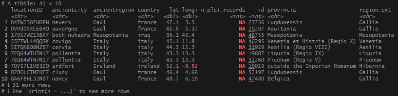
    Finally, I had a set of neat, tidy locations. It was time to do something with them. Mapping seemed like a logical next step – but where to start? The foundation of churches and dioceses was a data point that popped up often in my research, so I thought that would be a good place to jump in.

    In simple terms, a diocese or see, is the head of Catholic churches in a region, and is overseen by a Bishop. As Christianity grew, so did the establishment of churches, then dioceses to oversee them, and finally archdioceses, and patriarchal sees to oversee everything under them. There are many dioceses that were erected very early on, and indeed count apostles of Christ as their founders. An obvious example is Rome. The diocese is traditionally said to be founded and led by the first Pope, the apostle St. Peter, before his death in ~64.
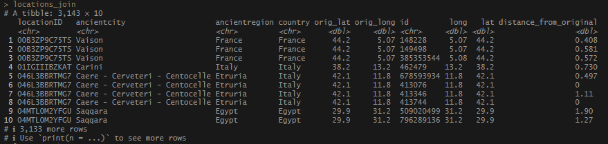
    In this post, I am not going to share the code or the data that I used to produce my locations list – mainly because it involves operations I have covered extensively (join and bind functions). As I said at the start, If you want to follow along, you just need a file or object that has individually identified longitude and latitude columns, or use one of the sets I link above.

    # This needs to be ran to prevent errors with rendering the world map below. This turns off 
    # spherical geometry package.
    sf_use_s2(FALSE)
    
    # Load packages.
    library(tidyverse)
    library(sf)
    
    # Read in your world shapefile. 
    # These were downloaded from https://www.naturalearthdata.com/
    world <- st_read("... directory where code resides... /ne_10m_admin_0_countries/ne_10m_admin_0_countries.shp")  
    • Load packages tidyverse and sf.
    • Use st_read() from the sf package to read in the shapefile (.shp).
    • Important: Keep the file structure from the .zip file in tact. The file folders need to reside in the same directory as your code for it to function correctly.

    Next, I had to do a little prepping of my data so it could be read by the plotting function I was going to apply. Again, the sf package provided the functions to get things in working order.

    # Check coordinates that the world map uses.
    st_crs(world)
    
    # Make sf object for plotting.
    diocese_sf <- diocese_1 %>% 
      dplyr::filter(status %in% c("Established","in_description","Erected")) %>% 
      rename("lon" = longi) %>% 
      dplyr::filter(!is.na(lat)) %>% 
      dplyr::select(locationID, lon, lat) %>% 
      st_as_sf(coords = c("lon", "lat")) %>% 
      st_set_crs(st_crs(world))
    • Filter my records only to the diocese dates that reflect the start or establishment of a diocese ("Established", "in_description", "Erected").
    • Other quick cleaning: fix the longitude column name so it can be read by the sf functions, filter out the NA values, and select only the necessary columns: locationID, lon, lat.
    • With st_as_sf(), I specify that I am using longitude and latitude coordinates.
    • Use st_set_crs() to match the coordinate system of world.

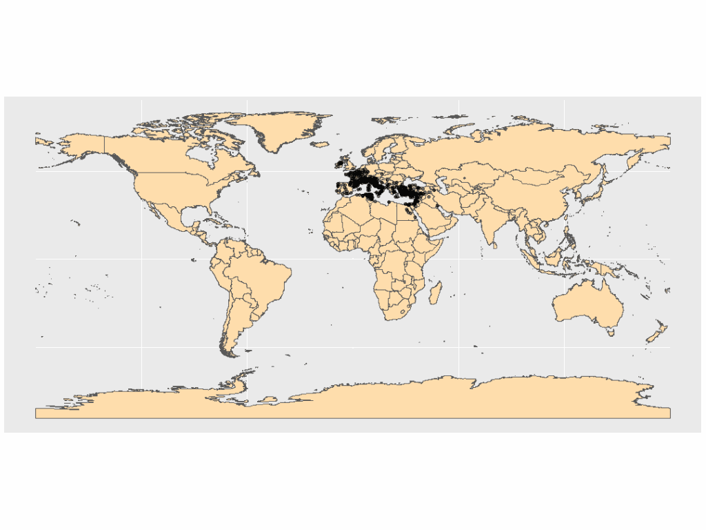
    I passed the new object into ggplot and used the geom_sf() function to render both the shapefile and my location data. The resulting plot was not helpful.

    Not helpful!

    I needed to crop the map. Finding my boundaries was easy, and the sf package had a cropping function that would constrain the map to a certain area. I just needed to find the min/max values of my coordinates, then use st_crop() to apply the boundaries.

    # Find min/max of my location data for cropping to the area that holds all of my points.
    diocese_1 %>% 
      filter(!is.na(lat)) %>% 
      summarize(min_lon = min(longi),
                max_lon = max(longi),
                min_lat = min(lat),
                max_lat = max(lat))
    
    # Create the cropped polygon object
    world_cropped <- st_crop(world,
            xmin = -10, xmax = 48, 
            ymin = 23, ymax = 57)
    
    • Filter the incomplete coordinates out of diocese_1 by removing NA values with !is.na(). Create a basic summary with the min and max of the lat and longi values.
    • Using st_crop(), create a cropped polygon object using the coordinates found in the previous step. I slightly decreased/increased the min/max values to give some breathing room to the points on the edges of the map

    Now plot!

    ggplot() +
      geom_sf(data = world_cropped,
              fill = "navajowhite") +
      geom_sf(data = diocese_sf,
              alpha = 0.5)
    • Call ggplot(). Here, I do not need to define aesthetics. X, Y values will come from diocese_sf.
    • With geom_sf(), add the world_cropped object as the first layer. I used navajowhite to color the land mass.
    • In the second geom_sf(), add the diocese_sf object. I adjusted the opacity to 50% with alpha = 0.5 to make the clustered points more visible.

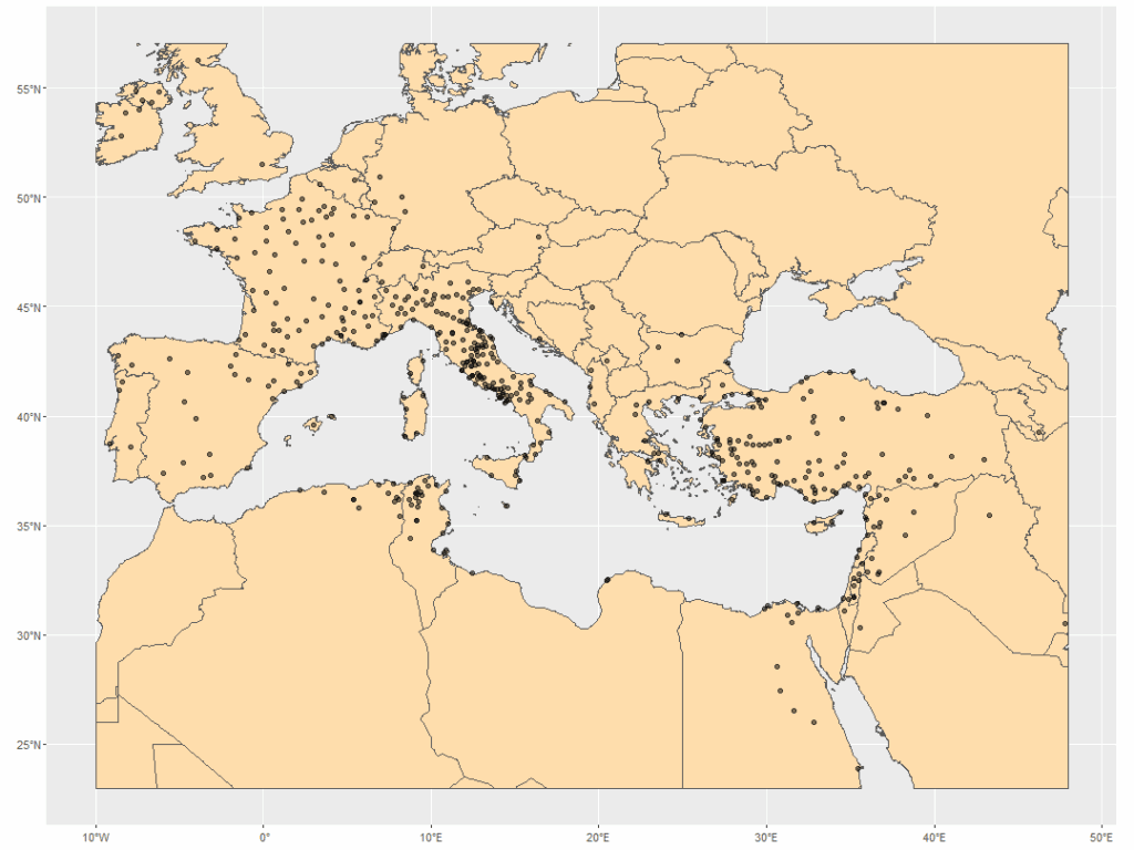
    Much better! I immediately saw some interesting patterns in my points – something to explore, next.

    Follow along script is on Github.

    • Cheney, David M. (2025) “Catholic-Hierarchy: Its Bishops and Dioceses, Current and Past.” Copyright David M. Cheney, 1996-2025. https://www.catholic-hierarchy.org/.
    • “CATHOLIC ENCYCLOPEDIA: Home.” (2025). https://www.newadvent.org/cathen/.
    • Pebesma, E., & Bivand, R. (2023). Spatial Data Science: With Applications in R. Chapman and Hall/CRC. https://doi.org/10.1201/9780429459016
    • “Natural Earth  – Free Vector and Raster Map Data at 1:10m, 1:50m, and 1:110m Scales.” (2025). https://www.naturalearthdata.com/.

  • Tangling with Location Names, part 2

    Once I had my long list of names, joining my no_matches set  was very easy. I used an inner_join() and pulled in any record from tris_data_long_clean that matches my locations, both in name and in country. I was able to snag several more records.

    tris_matches_2_no_matches <- no_matches %>% 
      mutate(ancientcity = str_to_lower(ancientcity),
             country = str_to_lower(country)) %>%
      inner_join(
        tris_data_long_clean,
        by = join_by(ancientcity == name,
                     country == country)) 
    • Apply str_to_lower() on both ancientcity and country. This helps standardize the name in case any random capitalizations exist, and assists in the inner_join().
    • inner_join() to match (exactly) on the name, and also the country, to ensure we have the right place. If there is no 1:1 match on name/country, then the record will be dropped. These locations will be re-joined later.
    41 more records – not bad!

    After this, I had 2 sets I wanted to bring together: locations_5km – the set joined by coordinates with Pleiades IDs; and then the new set generated from no_matches with TM IDs. I wanted to pull all of them together into one, tidy data frame. I remembered that Pleiades uses Trismegistos as one of their standard sources, and to keep things consistent, I decided to pull over the available TM ID’s from the Pleiades data. I also pulled over the Roman provincia, if it was available.

    The following code, as in the post before, is broken up, but is actually one long script, meant to be run all at once.

    # Start Script
    
    # Block 1
    # Bind the 2 data sets together by rows.
    locations_plei_and_tris <- locations_5km %>% 
      rename("plei_id" = id) %>% 
      select(-long,
             -lat) %>% 
      bind_rows(
        tris_matches_2_no_matches %>% 
          rename("orig_lat" = lat,
                 "orig_long" = longi,
                 "tris_id" = id)) %>% 
    • With locations_5km, I rename the ID column to plei_id to specify that it is the Pleiades ID.
    • Remove the long and lat column with select() – I only want to use my original coordinate values. I will keep the distance_from_original value for reference.
    • Join the 2 sets: locations_5km and tris_matches_2_no_matches, by row with bind_rows(). This will “stack” the rows, combining like columns together, and pulling over whatever columns that are not in common between the 2 sets, and filling them with NA values. Within the bind, I clean up some column names within tris_matches_2_no_matches/

    Next was a series of left_joins() to pull in the TM ID’s for the existing Pleiades ID’s I had and the provincia information for those ID’s.

      # Block 2
      left_join(
        pleiades_from_json_cleaned_tidied$pleiades_references %>% 
          filter(grepl("trismegistos", accessURI, ignore.case = T)) %>% 
          mutate(tris_id_extract = str_extract(accessURI, "[0-9]+")) %>% 
          select(id, tris_id_extract),
        by = join_by(plei_id == id)) %>% 
      # Block 3
      left_join(
        tris_data_long_clean %>% 
          select(id, 
                 provincia, 
                 country) %>% 
          mutate(id = as.character(id)) %>% 
          distinct(),
        by = join_by(tris_id_extract == id)
      ) %>% 
      # Block 4
      mutate(trismegistos_id = coalesce(as.character(tris_id), tris_id_extract),
             trismegistos_provincia = coalesce(provincia.x, provincia.y)) %>% 
      rename("country" = country.x) %>% 
      select(-provincia.x,
             -region_ext,
             -tris_id_extract,
             -provincia.y,
             -country.y,
             -tris_id) 
    
    # End script.
    locations_cited <- locations_master %>% 
      rename("orig_region" = ancientregion,
             "orig_country" = country) %>% 
      left_join(
        locations_plei_and_tris %>% 
        select(-ancientcity,
               -ancientregion,
               -country,
               -orig_lat,
               -orig_long),
        by = join_by(locationID == locationID))  
    • In the original locations_master, apply better names to reflect which source the region and country came from – assign with rename().
    • left_join() to the locations_plei_and_tris object that was just created. Inside the join, remove what would be redundant data. Any locationIDs that do not have a match will have NA values in both the plei_id and trismegistos_id fields.
    • Join the 2 sets by locationID. Store in the object locations_cited.

    Quick look at some of the records that didn’t come over. These will require some more research or fuzzy matching to sweep them up. Fortunately, there were only 109 orphaned records out of my original set of ~1,300.

    I also noticed that some of my locations independently pulled in a Pleiades ID and a TM ID, creating a duplicate row in some cases. I will have to figure out how suppress that in future iterations.

    Despite that, I decided that this is really, really good locations data set, and that it would be OK to pause here and move onto something else. I was interested in taking one of my data sets, linking it to my locations data, and plotting it on a world map. Fortunately, I had a lot of other records tied to these locationID’s where I could do that.

  • Tangling with Location Names, part 1

    pleiades_from_json_cleaned_tidied #Cleaned data from Pleiades JSON data
    locations_5km  #Locations within 5km of the original coordinates.
    locations_master #My original locations list.
    no_matches #Locations that did not find a match during the fuzzyjoin.
    # Start script
    
    # Block 1
    # Start big cleanup of tris data
    tris_data_long_clean <- trismegistos_all_export_geo %>% 
      as_tibble() %>% 
      select(id,
             provincia,
             country,
             name_latin,
             name_standard,
             full_name) %>% 
     separate_wider_delim(
        full_name,
        delim = " - ",
        names = c("country_region_ext","city_ext"),
        too_many = "merge",
        too_few = "align_start") %>% 
    • Note: trismegistos_all_export_geo is the object loaded from the TM .csv file referenced above. From this, use select() to pick only the necessary variables/columns.
    • Start the first separation. It looks like there is only one initial break marked with space-underscore-space ( – ), which will be the delimiter in delim = . The next steps are done inside the separation.
      • Specify the full_name column, and the delimiter.
      • Separate column into 2 columns: "country_region_ext" and "city_ext".
      • In the event there is more or less data than can fit in 2 columns, what to do with those values . If there are more than 2 (too_many), the remaining values are merged into the 2nd column with separators in tact. If there is 1 value (too_few), it will be placed in country_ext, the start of the created columns.
    # Block 2
      separate_wider_delim(
        country_region_ext,
        delim = ",",
        names = c("country_ext","region_ext"),
        too_many = "merge",
        too_few = "align_start") %>%
    • Do another separation, just like above, this time breaking country_region_ext at the commas to get the country and regions alone.
    #Block 3
    mutate(city_ext = str_replace_all(city_ext, " \\[", "(")) %>% 
    • Mutate the city_ext column using str_replace_all(). The inconsistent bracket vs. parenthesis make the next separation difficult. So, I want to replace left-brackets with left-parenthesis. The \\ with the left-brackets are escape characters, and need to be used when working with certain characters inside R.*
    # Block 4
      separate_wider_delim(
        city_ext,
        delim = "(",
        names = c("city_ext_1","city_ext_2"),
        too_many = "merge",
        too_few = "align_start") %>%
    • Yet more separations. Just like 2 and 3 above, this time breaking city_ext at the parenthesis. This allows me to get at the appended information I discussed above.
    # Block 5
      separate_wider_delim(
        name_latin,
        delim = " - ",
        names = paste0("tris_latin_", 1:25),
        too_many = "merge",
        too_few = "align_start") %>% 
      select(where(~ !all(is.na(.))),
             -country_ext) %>% 
    • Some of these names have, like, 20+ delimiters (all consistent, thank God!), so I separate them into a large number of columns – more than I probably need. To do this, I use paste0() to affix a “tris_” to the columns, then a sequence of 1-to-whatever I want. Here, 25 – seemed like plenty. This results in 25 columns named tris_1 through tris_25, plenty of room for separation.
    • Because not every place will have 25 different names, those extra columns will be filled entirely with NA values. Here, the select() function looks across all of my columns, and filters out those where all of the values in the column are NA. At the same time, I remove the country_ext, as it is truly redundant.
    # Block 6
      pivot_longer(!c(id, provincia, region_ext, country),
                   names_to = "source_seq",
                   values_to = "name") %>% 
    • Pivot this (now) very wide list into one long list using pivot_longer(). Pivot everything except id, provincia, region_ext, and country. Save the column names into a new column called "source_seq" and the city names into "name".
    # Block 7
      mutate(name = str_trim(str_to_lower(name)),
             region_ext = str_trim(region_ext),
             name = if_else(name == "", NA, name),
             country = str_to_lower(country),
             name = str_replace_all(name, "\\)", "")) %>% 
      filter(!is.na(name)) %>% 
      select(-source_seq) %>% 
      distinct() %>% 
      relocate(name, .after = id)
    
    #End script
    • Apply several mutations to clean up some of the columns:
      • Trim the whitespace with str_trim() in name and region_ext (the separation process can generate a lot of it). I also converted the names to lowercase with str_to_lower() for standardization.
      • Apply an if_else() – if the name is an empty field (represented by “”), then replace it with an NA, so it can easily be filtered out later. Else, leave whatever is in place.
      • Convert country to lower case. This should make the country names more standardized – important for joining later.
      • Replace the random right-parenthesis artifacts from the separation with blanks.
    • Filter out any NA values in the name column.
    • Remove the source_seq column. It is not needed anymore.
    • distinct() to condense all identical records into one, so each record is distinct.
    • Finally, move the name column so it is right after the id – easier for me to read.

    TM data before:

    R screenshot

    TM data after:

    So much better.

    The final step to all of this was using this list to join the no_matches records to see if I could sweep in some of the TM sources where I did not have Pleiades. I also wanted to pull the TM ID’s from the Pleiades data and put them into my set. Since this script was so long, I stored the results in an object (tris_data_long_clean) and saved it as an .rds file for safe keeping.

    # Save
    saveRDS(tris_data_long_clean, paste0(objects_directory,"tris_data_long_clean.rds"))
  • Finding Location Information with fuzzyjoin

    Now that I had some good location data, I wanted to use my coordinates to join the Pleiades data and see what …stuff is in the immediate area of my locations. To do this, I used a package called fuzzyjoin, which has a function called geo_inner_join (and geo_right_join, geo_left_join, etc.)* which allows you to join 2 sets of coordinates based on distance – either kilometers or miles. I decided that 2km (1.24 m) would be a good place to start. The joining took several seconds and produced a long data set with each identified each Pleiades ID on its own line.

    # Read in object.
    locations_master  <- readRDS(paste0(objects_directory,"locations_reversed_joined.rds"))
    
    
    #attestations based on lat/long - this will take several seconds.
    locations_join <- locations_master %>% 
      filter(!is.na(lat)) %>% 
      rename("orig_lat" = lat,
             "orig_long" = longi) %>% 
      geo_inner_join(
        pleiades_from_json$pleiades_locations %>% 
          filter(!is.na(long)),
        by = c("orig_long" = "long",
               "orig_lat" = "lat"),
        unit = c("km"),
        max_dist = 2,
        distance_col = "distance_from_original"
        )
    • Filter out the NA values in lat (which should remove any incomplete coordinates).
    • Rename my existing lat/long columns so that I can easily identify which frame they belong to after I perform my join.
    • Perform the geo_inner_join.
      • This will look at the list pleiades_from_json$pleiades_locations and filter out any incomplete coordinates.
      • Join the 2 sets: my orig_long to Pleiades’ long, and my orig_lat to Pleiades’ lat.
      • unit = c("km") – use kilometers (km) for the units.
      • max_dist = 2 – include all matches within 2km of my coordinates.
      • Put the distance value in a column called “distance_from_original“.
    • Save it all in an object called locations_join.
    • * – the inner_join indicates that the script it will keep only the records that match the requirements of the join.

    I forgot that I didn’t have names paired with those coordinates I pulled from the JSON file. Good thing I have that object at the ready. I decided to utilize the title value to give me the basic name of the record associated with the Pleiades ID’s. The pleiades_full_json$@graph$names list has every single variation on a name in Pleiades, and is a little beyond what I needed (for the moment!) I made a set of ID’s-to-titles and saved it to my pleiades_from_json_cleaned_tidied object to keep it handy. Then I joined it to locations_join.

    # As before:
    plei_ids <- pleiades_full_json$`@graph`$id
    
    # Grab titles.
    plei_titles <- pleiades_full_json$`@graph`$title
    
    # Pull id's and titles together.
    pleiades_titles <- tibble(
      id = plei_ids,
      plei_title = plei_titles
    ) 
    
    # Save these to the big list real quick.
    pleiades_from_json_cleaned_tidied[["pleiades_titles"]] <- pleiades_titles
    
    # Save the list.
    saveRDS(pleiades_from_json_cleaned_tidied, paste0(objects_directory, "pleiades_from_json_cleaned_tidied.rds"))
    
    # Join the titles to the joined set so we can see the names of the matched records.
    locations_full_join_w_titles <- locations_join %>% 
      left_join(
        pleiades_titles,
        by = join_by(id == id))
    • Extract titles list and store in plei_titles.
    • Pull both sets together into one tibble called pleiades_titles.
    • Save this new set to the existing pleiades_from_json_cleaned_tidied list.
    • Join the pleiades_titles to locations_join using the id column in both data sets.

    Cool. Next I wanted to see which locations had the most attestations based on these coordinates.

    locations_full_join_w_titles %>% 
      group_by(
        ancientcity,
        country,
        orig_lat,
        orig_long
      ) %>% 
      summarize(n_plei_records = n_distinct(id)) %>% 
      arrange(desc(n_plei_records))
    • Aggregate the data with summarize() and count each distinct id in each group. Sort it so you can see the highest number of ID’s at the top. with arrange(desc()).

    There were some famous, well attested sites that came up, but where was Rome? Or Constantinople? I decided to widen my geo_inner_join to 5km (3.11 miles), then aggregate.

    locations_5km <- locations_master %>% 
      filter(!is.na(lat)) %>% 
      rename("orig_lat" = lat,
             "orig_long" = longi) %>% 
      geo_inner_join(
        pleiades_from_json$pleiades_locations %>% 
          filter(!is.na(long)),
        by = c("orig_long" = "long",
               "orig_lat" = "lat"),
        unit = c("km"),
        max_dist = 5,
        distance_col = "distance_from_original"
      )
    
    locations_5km %>% 
    group_by(
      ancientcity,
      country,
      orig_lat,
      orig_long
    ) %>% 
      summarize(n_plei_records = n_distinct(id)) %>% 
      arrange(desc(n_plei_records))

    How about 10km? (Note: this code is all run together and goes right to the summary.)

    locations_master %>% 
      filter(!is.na(lat)) %>% 
      rename("orig_lat" = lat,
             "orig_long" = longi) %>% 
      geo_inner_join(
        pleiades_from_json$pleiades_locations %>% 
          filter(!is.na(long)),
        by = c("orig_long" = "long",
               "orig_lat" = "lat"),
        unit = c("km"),
        max_dist = 10,
        distance_col = "distance_from_original"
      ) %>% 
      group_by(
        ancientcity,
        country,
        orig_lat,
        orig_long
      ) %>% 
      summarize(n_plei_records = n_distinct(id)) %>% 
      arrange(desc(n_plei_records))

    More obscure cities with tons of records. It also took a little longer to perform the join. The wider the search, the more location overlap I was likely to have. I decided that 5km might be the highest tolerance to apply in my search. And, at some point, it might be interesting to check out which ID’s my records shared in common.

    Portion of the main Pleiades record for Dura with all associated sites plotted.
    All these references!

    Then, I wanted to check on the locations that did not produce any matches.

    # Who did not have matches?
    no_matches <- locations_master %>% 
      left_join(locations_5km %>% 
        group_by(
          locationID) %>% 
          summarize(n_plei_records = n_distinct(id),
                    .groups = "drop"),
        by = join_by(locationID == locationID)) %>% 
      filter(is.na(n_plei_records))
    • Take my original locations_master and left_join() to the 5km data set. Since we just want a quick check of number of records, inside that left_join(), group the records to locationID and then get the total number of distinct Pleiades ID’s per locationID.
    • Join by the locationID in each data set.
    • filter(is.na(n_plei_records)) to focus on the records that did not have any ID’s found for it’s coordinates.

    Finally, save the locations_5km and the locations_master objects for the next round of matches.

    saveRDS(locations_5km, paste0(objects_directory,"locations_5km.rds"))
    saveRDS(locations_master, paste0(objects_directory,"locations_master.rds"))
    saveRDS(no_matches, paste0(objects_directory,"no_matches.rds"))
    

    Robinson D (2025). fuzzyjoin: Join Tables Together on Inexact Matching. R package version 0.1.6, https://github.com/dgrtwo/fuzzyjoin.

  • Reading in JSON data with jsonlite

    • Use read.csv() to read in the Trismegistos .csv file and save it as an object called trismegistos_all_export_geo.
    • Use read_json() from the jsonlite package to read in the .json file. This was a huge file and took between 10-15 minutes to finish loading. Save this as an object called pleiades_full_json.
      • simplifyDataFrame = T, puts lists containing only records (JSON objects) into a single data frame;
      • flatten = T, flattens nested data frames into a single data frame if possible;
    • Roger Bagnall, et al. (eds.), Pleiades: A Gazetteer of Past Places, 2016, <http://pleiades.stoa.org/> [Accessed: February 17, 2016].
    • H. Verreth, A survey of toponyms in Egypt in the Graeco-Roman period (Trismegistos Online Publications, 2), Leuven: Trismegistos Online Publications, 1253 pp.
    • Ooms J (2014). “The jsonlite Package: A Practical and Consistent Mapping Between JSON Data and R Objects.” arXiv:1403.2805 [stat.CO]https://arxiv.org/abs/1403.2805.

  • Using tidygeocoder’s reverse_geocode()

    Way back when I was actively collecting my data, I was obsessed with making sure that the places associated with my entries both existed, and were locatable. I spent a lot of time tracking down place names, alternative names, modern names, whatever was out there. Eventually, the list became very long, with tons of duplicate entries (like, did you know that a lot of early Christian events took place in Rome? Who knew!) I realized I had to organize this nonsense, and decided to build a mySQL database to store it all. I took all my city/country locations and consolidated them to one-record-per-location, assigned a unique ID for that particular place, then created a table for it in database. This is currently how all of my location data exists and is the most up-to-date.

    I wanted to grab my latitudes (lat) and longitudes (longi) and feed them into the reverse_geocode() function, then apply some other useful arguments. I stored it all in an object called “rev_geo“. The whole thing looked like this:

    When reverse geocode finished, I wanted to check the matches. I created a quick a script to check my work and see which countries matched up.

    All of my entries were instances where the names were different, but correct (i.e: Britain vs. United Kingdom); regions that used to stretch through many countries (i.e.: Roman Mauretania), and some of the cities rest on the borders. I thought it looked good and decided to pause. Since the geocode took awhile, I wanted to save it so that I had it on hand for the next steps. I stashed it in my “objects” directory where I save all my .rds files.

    Cambon J, Hernangómez D, Belanger C, Possenriede D (2021). tidygeocoder: An R package for geocoding. Journal of Open Source Software, 6(65), 3544, https://doi.org/10.21105/joss.03544 (R package version 1.0.5)